How To Find A Table In Excel

Everything You Need to Know About Excel Tables

In this post, we're going to acquire everything there is to know about Excel Tables!

Yep, I hateful everything and at that place's a lot.

This postal service will tell you about all the awesome features Excel Tables have and why you should start using them.

What is an Excel Tabular array?

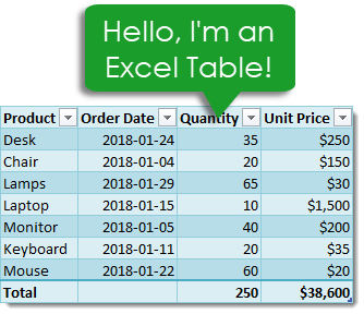
Excel Tables are containers for your data.

Imagine a house without whatever closets or cupboards to shop your things, information technology would be anarchy! Excel tables are similar closets and cupboards for your information, they assist to contain and organize data in your spreadsheets.

In your business firm, you might put all your plates into one kitchen closet. Similarly, you might put all your client information into one Excel table.

Tables tell excel that all the data is related. Without a table, the simply thing relating the data is proximity to each other.

Ok, so what's so great about Excel Tables other than being a container to organize data? A lot really. This post will tell you lot near all the awesome features tables have and should convince you to start using them.

Video Tutorial

The Parts of a Tabular array

Throughout this post, I'll be referring to various parts of a tabular array, and so information technology's probably a adept idea that we're both talking near the aforementioned affair.

This is the Column Header Row. It is the first row in a table and contains the column headings that place each cavalcade of information. Column headings must be unique in the table, they cannot be blank and they cannot contain formulas.

This is the Trunk of the table. The body is where all the information and formulas live.

This is a Row in the tabular array. The torso of a table can contain one or more than rows and if you effort to delete all the rows in a tabular array a single blank row will remain.

This is a Cavalcade in the table. A table must contain at least one column.

This is the Total Row of the table. Past default, tables don't include a total row but this feature can exist enabled if desired. If it's enabled, it will be the last row of the table. This row can contain text, formula or remain blank. Each cell in the total row will accept a drib downwardly menu that allows selection of various summary formula.

Create a Table from the Ribbon

Creating an Excel Table is really piece of cake. Select whatsoever cell inside your data and Excel will approximate the range of your data when creating the table. Yous'll be able to confirm this range later on on. Instead of letting Excel judge the range you can also select the entire range of information in this stride.

With the active cell inside your data range, go to the Insert tab in the ribbon and press the Table button constitute in the Tables section.

The Create Tabular array dialog box volition pop up. Excel guesses the range and you lot can adjust this range if needed using the range selector icon on the right hand side of the Where is the data for your tabular array? input field. You tin also conform this range by manually typing over the range in the input field.

Checking the My table has headers box will tell Excel the first row of information contains the column headers in your table. If this is unchecked Excel will create generic column headers for the table labelled Column 1, Column ii etc…

Press the Ok push when you're satisfied with the data range and table headers check box.

Congratulations! You now accept an Excel table and your data should await something like the above depending on the default style of your tables.

Contextual Table Tools Design Tab

Whenever you select a cell inside a table, you volition notice a new tab appear in the ribbon labelled Tabular array Tools Blueprint. This is a contextual tab and merely appears when a tabular array is selected. When the agile jail cell moves outside the table, the tab will disappear again.

This is where all the commands and options related to tables will live. This is where you'll exist able to name your table, discover table related tools, enable or disable tabular array elements and change your table'south style.

Create a Tabular array with a Keyboard Shortcut

You can besides create a table using a keyboard shortcut. The procedure is the aforementioned as described to a higher place but instead of using the Table push in the ribbon you can printing Ctrl + T on your keyboard. It'due south easy to remember since T is for Table!

There is actually another keyboard shortcut that you lot tin can employ to create tables, Ctrl + 50 volition likewise do the same thing. This is a legacy from when tables were chosen lists (L is for Listing).

Name a Table

Anytime you create a new table Excel will give it an initial generic name starting with Table1 and increasing sequentially. Yous should e'er rename your tabular array with a descriptive and short name.

Not all names are immune. At that place are a few rules for a table name.

Each table must have a unique name inside a workbook.
You tin merely use messages, numbers and the underscore character in a table proper noun. No spaces or other special characters are allowed.
A table proper noun must brainstorm with either a letter or an underscore, it can not brainstorm with a number.
A tabular array name can take a maximum of 255 characters.

Select any cell inside your table and the contextual Table Tools Design tab will announced in the ribbon. Within this tab you tin find the Tabular array Proper noun under the Properties section. Type over the generic name with your new proper name and press the Enter push when finished to ostend the new name.

Rename a Table

Renaming a tabular array y'all've already named is the aforementioned process as naming a tabular array for the starting time time. If you retrieve virtually it, when you first proper noun a table you're really renaming it from the generic name of Table1 to a new proper noun.

So go back to the Table Tools Design tab and type your new proper noun over the old i in the Table Proper noun and press Enter. Easy, and the proper name is changed.

Changing your table proper name this mode requires navigating to your tabular array and selecting a jail cell within it, then information technology tin can be dull if you need to rename a lot of tables across unlike sheets in your workbook. Instead, yous can change any of your table names without going to each tabular array using the Name Manager.

Go to the Formula tab and printing the Proper name Manager push in the Defined Names section. You'll exist able to see all your named objects here. The table objects volition have a small table icon to the left of the name. You tin can filter to show only the table objects using the Filter button in the upper right hand corner and selecting Table Names from the options.

Yous can so edit whatever name by selecting the item and pressing the Edit button. You'll be able to modify the name and add some comments to describe the information in your table.

Navigate Tables with the Name Box

You can hands navigate to any table in your workbook using the name box the the left of the formula bar. Click on the small pointer on the right side of the proper noun box and you volition see all table names in the workbook listed. Click on any of the tables listed and yous will exist taken to that table.

Catechumen a Tabular array Back to a Normal Range

Ok, you changed your mind and don't want your data inside a table anymore. How do you catechumen it back into a regular range?

If changing it to a table was the last thing yous did, Ctrl + Z to undo your concluding activeness is probably the quickest way.

If it wasn't the last thing you lot did, then you're going to need to apply the Convert to Range command establish in the Table Tools Design tab under the Tools department.

You'll exist prompted to ostend that you lot actually want to convert the table to a normal range. Noooooo, don't do it, tables are awesome!

If you click on yes, then all the awesome benefits from tables will be gone except for the formatting design. Yous'll need to manually articulate this from the range if y'all want to get rid it. You can do this by going to the Abode tab then pressing the Clear button found in the Editing section, and so selecting Clear Formats.

This tin can likewise exist done from the right click menu. Right click anywhere in the table and select Tabular array from the menu and then Catechumen to Range.

Select the Entire Cavalcade

If your data is not inside a table and so selecting an entire cavalcade of the data can be difficult. The usual way would be to select the commencement cell in the column and then hold Ctrl + Shift and so press the Down arrow primal. If the column has bare cells, then you might demand to press the Down arrow key a few times until you reach the end of the data.

The other option is to select the starting time prison cell and then use the scroll bar to whorl to the terminate of your data then agree the Shift fundamental while you select the last column.

Both options tin can be tedious if yous have a lot of information or in that location are a lot of blanks cells in the information.

With a table, you lot can easily select the entire column regardless of blank cells. Hover the mouse cursor over the column heading until it turns into a small arrow pointing downward then left click and the unabridged column will be selected. Left click a second fourth dimension to include the column heading and any total row in the selection.

Some other way to apace select the entire column is to identify the active jail cell cursor on whatever cell in the column and press Ctrl + Infinite. This will select the entire column excluding the cavalcade header and full row. Press Ctrl + Space once again to include the column headers and total row.

Select the Entire Row

Selecting the entire row is merely as easy. Hover the mouse cursor over the left side of the row until it turns into a small pointer pointing left then left click and the entire row will be selected. This works on both the column heading row and total row.

Another way to quickly select the entire row is to place the active prison cell cursor on any cell in the row and printing Shift + Space.

Select the Entire Table

Information technology'southward also possible to select the entire table and in that location are a couple different means to practice this.

You tin place the active cell cursor within the table and press Ctrl + A. This will select the unabridged torso of the table excluding the column headers and total row. Printing Ctrl + A again to include the cavalcade headers and full row.

Hover the mouse over the tiptop left mitt corner of the table until the cursor turns into a minor black diagonal correct and downwards pointing arrow. Left click one time to select only the body. Left click a second fourth dimension to include the header row and full row.

You tin also select the table with the mouse. Place the active cell inside the table and then hover the mouse cursor over whatsoever edge of the tabular array until it turns into a 4 way directional arrow then left click. This will also select the cavalcade headers and full row.

Select Parts of the Table from the Correct Click Menu

You can as well select rows, columns or the entire table using the correct click bill of fare. Correct click anywhere on the row or column you want to select then choose Select and option from the 3 options available.

Add a Total Row

You can add a total row which allows you to display summary calculations in the final row of your table.

Adding summary calculations at the bottom of your data can be dangerous as they might cease upwardly getting included by accident in a pivot tabular array using the information. This is some other advantage of tables, as the total row won't be included in any pivot tables created with the table.

To enable the full row, go to the Tabular array Tools Design tab and check the Total Row box establish in the Table Way Options section.

You can temporarily disable the total row without losing the formulas you added to it. Excel will remember the formulas yous had and they will appear when you enable it again.

Each cell in the total row has a drop down menu that allows yous to pick various aggregating functions to summarize the column of data to a higher place.

Yous can besides enter your own formulas. I've entered a SUMPRODUCT formula in the Unit Price full to sum the Quantity ten Unit of measurement Price to calculate a total sale amount. Formulas don't have to return a number, they tin also be text results.

Constant numerical or text values are likewise allowed anywhere in the total row. In fact the leftmost column will usually contain the text Total past default.

Add a Total Row with a Right Click

You can also add the total row with a right click. Right click anywhere on the tabular array and the choose Tabular array and Total Row from the carte du jour.

Add a Total Row with a Keyboard Shortcut

Some other way to quickly add the total row is to identify the active jail cell cursor inside your table and use the Ctrl + Shift + T keyboard shortcut.

Disable the Column Header Row

The column header row is enabled by default, merely you lot can disable it. This doesn't delete the column headers, information technology's essentially similar hiding them every bit you will withal reference columns based on the cavalcade header name.

Become to the Tabular array Tools Design tab and uncheck the Total Row box constitute in the Tabular array Style Options section.

Add together Bold Format to the Kickoff or Last Columns

You tin enable a bold formatting on either your first or last column to highlight it and draw attention to them over other columns.

Go to the Table Tools Design tab and check either of the First Cavalcade or Last Column boxes (or both) constitute in the Table Style Options section.

Add Banded Rows or Columns

Banded rows are already enabled by default, but y'all can turn them off if you want. Banded columns are disabled by default, so you demand to enable them if you lot want them.

To enable or disable either, go to the Table Tools Design tab and check or uncheck the Banded Rows or Banded Columns boxes plant in the Tabular array Style Options section.

I by and large notice banded rows are the most useful and if you enable banded columns at the same time, the table starts to look a little messy. I recommend ane or the other and non both at the same fourth dimension.

Tabular array with no banded rows or columns.
Table with banded rows only.
Table with banded columns only.
Table with both banded rows and columns.

Table Filters

By default, the tabular array filters selection is enabled. You tin disable them from the Table Tools Blueprint tab past unchecking the Filter Push box found in the Table Style Options department.

You can as well toggle the filters on or off from the agile table by using the regular filter keyboard shortcut of Ctrl + Shift + L.

If you left click on any of the filters, it will bring upward the familiar filter carte du jour where you can sort your table and apply various filters depending on the blazon of data in the column.

The great thing most table filters is you can have them on multiple tables in the same sheet simultaneously. You will need to be careful though as filtered items in one table will affect the other tables if they share common rows. You can only have one set of filters at a time in a sheet of information without tables.

Total Row with Filters Applied

When you select a summary function from the driblet downwards card in the total row, Excel will create the respective SUBTOTAL formula. This SUBTOTAL formula ignores hidden and filtered items. And so when you filter your table these summaries will update accordingly to exclude the filtered values.

Annotation that the SUMPRODUCT formula in the Unit of measurement Toll column still includes all the filtered values while the SUBTOTAL sum formula in the Quantity column does not.

Column Headers Remain Visible When Scrolling

If you scroll down while the active cell is in a table, its column headers will remain visible along with the filter buttons. The table'southward cavalcade headings will get promoted into the sheet'due south cavalcade headings where we would normally see the alphabetic cavalcade name.

This is extremely handy when dealing with long tables equally you lot won't demand to scroll back up to the top to see the cavalcade name or utilize the filters.

Automatically Include New Rows and Columns

If you type or copy and paste new information into the cells directly below a table, they will automatically be absorbed into the tabular array.

The aforementioned thing happens when you type or copy and paste into the cells directly to the right of a table.

Automatically Fill Formulas Downwards the Entire Cavalcade

When you enter a formula inside a tabular array information technology will automatically fill the formula down the entire column.

Even when a formula has already been entered and y'all add new data to the row directly below the table whatever existing formulas will automatically fill.

Editing an existing formula in any of the cells will also update the formula in the entire column. You'll never forget to copy and paste downwardly a formula again!

Turn Off the Auto Include and Car Fill up Settings

You can plow off the feature that automatically adds new rows or columns and fills downwards formulas.

Get to the File tab and select Options. Choose Proofing and so press the AutoCorrect Options push button. Navigate to the AutoFormat As You Blazon tab in the AutoCorrect dialog box.

Unchecking the Include new rows and columns in table pick allows you to blazon directly underneath or to the right of a table without it absorbing the cells.

Unchecking the Fill formulas in tables to create calculated columns choice means the formulas in a table will no longer automatically fill down the cavalcade.

Resize with the Handle

Every tabular array comes with a Size Handle found in the lesser rightmost cell of the tabular array.

When yous hover the mouse over the handle, the cursor volition turn into a double-sided diagonally slanting arrow and you can so click and drag to resize the table. Yous can either expand or contract the size. Information volition be captivated into the table or removed from information technology appropriately.

Resize with the Ribbon

You tin likewise resize the tabular array from the ribbon. Become to the Tabular array Tools Design tab and press the Resize Table command in the Backdrop section.

The Resize Table dialog box volition pop upwards and you'll be able to select a new range for your table. Use the range selector icon to select a new range. You lot can select either a larger or smaller range, but The table headers will need to remain in the same row and the new table range must overlap the quondam tabular array range.

Add a New Row with the Tab Key

You can add a new blank row to a table with the Tab key. Identify the active prison cell cursor inside the tabular array on the cell containing the sizing handle and press the Tab key.

The tab key human action like a carriage render and the active prison cell is taken to the rightmost jail cell on a new line that's added directly below.

This is a handy shortcut to know considering when the full row is enabled, it's not possible to add a new row by typing or copying and pasting data direct below the table.

Insert Rows or Columns

You can insert extra rows or columns into a tabular array with a right click. Select a range in the table and correct click then choose Insert from the menu. You can then either choose to insert Table Columns to the Left or Table Rows Above.

Table Columns to the Left volition insert the number of columns selected to the left of the selection and the number of rows in the option is ignored.

Table Rows In a higher place volition insert the number of rows selected only above the selection and the number of columns in the option is ignored.

Delete Rows or Columns

Deleting rows or columns has a like story to inserting them. Select a range in the tabular array and right click then choose Delete from the carte. Yous tin can so either choose to delete Table Columns or Tabular array Rows.

Formats in a Table Automatically Apply to New Rows

When you add new data to your tabular array, you don't demand to worry well-nigh applying formatting to match the rest of the data above. Formatting will automatically make full down from above if the formatting has been applied to the entire column.

I'm not just talking about the table style formats. Other formatting like dates, numbers, fonts, alignments, borders, conditional formatting, prison cell colours etc. will all automatically make full downwards if they've been practical to the whole column.

If you've formatted all your numbers as a currency in a cavalcade and y'all add new data, it likewise volition go the currency format applied to information technology.

You lot never need to worry almost inconsistent formatting in your data.

Add a Slicer

You tin can add together a slicer (or several) to a table for an easy to employ filter and visual way to see what items the table is filtered on.

Go to the Table Tools Design tab and press the Insert Slicer button found in the Tools section.

Change the Style

Changing the styling of a tabular array is quick and like shooting fish in a barrel. Go to the Tabular array Tools Pattern select a new way from the selection institute in the Tabular array Styles section. If you left click the small downwardly arrow on the right manus side of the styles palette, information technology will aggrandize to show all available options.

These table styles apply to the whole table and will also apply to any new rows or columns added later on.

There are many options to cull from including light, medium and dark themes. As you hover over the various selections, you'll be able to see a live preview in the worksheet. The fashion won't actually change until you lot click on one though.

You can even create your own New Tabular array Style.

Fix a Default Table Mode

You can set any of the styles available every bit the default so that when you create a new table y'all don't need to change the style. Right click on the style you lot want to set as the default and so choose Set As Default from the bill of fare.

Unfortunately, this is a workbook level setting and will only affect the electric current workbook. You will need to set the default for each workbook you create if you don't want the application default option.

Only Impress the Selected Table

When you identify the active prison cell cursor within a table and and so try to print, there is an option to only print the selected table. Go to the Impress carte du jour screen by either going to the File tab and selecting Print or using the Ctrl + P keyboard shortcut, then select Print Selected Table in the settings.

This will remove whatever items from the print area that are not in the table.

Structured Referencing

Tables come with a useful feature called structured referencing which helps to make range references more readable. Ranges within a table tin exist referred to using a combination of the table name and column headings.

Instead of seeing a formula like this =SUM(D3:D9) you might see something like this =SUM(Sales[Quantity]) which is much easier to understand the pregnant of.

This is why naming your table with a brusk descriptive proper noun and column headings is of import every bit it will amend the readability of the structured references!

When you reference specific parts of a table, Excel will create the reference for you so you don't need to memorize the reference construction but it will assist to understand it a bit.

Structured references tin can contain upwards to three parts.

This is the table name. When referencing a range from inside the table this function of the reference is not required.
These are range identifiers and place certain parts of the reference for a table like the headers or total row.
These are the cavalcade names and will either be a single column or a range of columns separated by a full colon.

Case of structured References for a Row

=Sales[@[Unit of measurement Price]] will reference a single cell in the body.
=Sales[@[Product]:[Unit Price]] will reference role of the row from the Product column to the Unit Price column including all columns in between.
=Sales[@] will reference the full row.

Case of Structured References for Columns

=Sales[Unit Cost] will reference a single column and only include the body.
=Sales[[#Headers],[#Data],[Unit Price]] will reference a unmarried column and include the column header and body.
=Sales[[#Data],[#Totals],[Unit Price]] will reference a single column and include the body and total row.
=Sales[[#All],[Unit Price]] will reference a single cavalcade and include the column header, trunk and full row.

Example of Structured References for the Total Row

=Sales[#Totals] will reference the entire total row.
=Sales[[#Totals],[Unit of measurement Price]] will reference a cell in the full row.
=Sales[[#Totals],[Production]:[Unit Cost]] will reference part of the full row from the Product column to the Unit Price column including all columns in between.

Example of Structured References for the Column Header Row

=Sales[#Headers] will reference the entire cavalcade header row.
=Sales[[#Headers],[Order Date]] volition reference a jail cell in the column header row.
=Sales[[#Headers],[Product]:[Unit Toll]] will reference part of the column header row from the Product cavalcade to the Unit of measurement Cost column including all columns in between.

Example of Structured References for the Table Torso

=Sales will reference the entire body.
=Sales[[#Headers],[#Data]] will reference the entire column header row and body.
=Sales[[#Information],[#Totals]] volition reference the unabridged torso and total row.
=Sales[#All] will reference the unabridged column header row, trunk and full row.

Using Intellisense

One of the great things almost a table is the structured references will appear in Intellisense menus when writing formulas. This means you can easily write a formula using the structured references without remembering all the fields in your tabular array.

After typing the kickoff letter of the alphabet of the tabular array name, the IntelliSense bill of fare volition show the tabular array name amid all the other objects starting with that letter. You tin can use the arrow keys to navigate to information technology and then press the Tab key to autocomplete the table name in your formula.

If you want to reference a part of the table, you can then type a [ to bring up all the available items in the tabular array. Over again, yous tin navigate with the arrow keys and and so use the Tab fundamental to autocomplete the field name. Then you can close the particular with a ].

Plow Off Structured Referencing

If you're not a fan of existence forced to use the structured referencing system, then you can plow information technology off. Any formulas that have been entered using the structured referencing volition remain and they volition still work the same. Yous'll too still exist able to use structured references, Excel but won't automatically create them for you.

To turn it off, go to the File tab and then select Options. Cull Formulas on the side pane then uncheck the Apply tabular array names in formulas box and press the Ok push.

Summarize with a PivotTable

You tin can create a pivot table from your tabular array in Table Tools Design tab, press the Summarize with PivotTable button found in the Tools department. This volition bring up the Create PivotTable window and y'all can create a pivot table every bit usual.

This is the same as creating a pivot table from the Insert tab and doesn't give any actress options specific to tables.

Remove Duplicates from a Table

You lot tin create remove duplicate rows of data from your table in Table Tools Design tab, press the Remove Duplicates button found in the Tools department. This will bring up the Remove Duplicates window and delete duplicate values for one or more columns in the table.

This is the same as removing duplicates from the Data tab and doesn't give any extra options specific to tables.

About the Author

John MacDougall

John is a Microsoft MVP and freelance consultant and trainer specializing in Excel, Power BI, Power Automate, Power Apps and SharePoint. You can find other interesting manufactures from John on his blog or YouTube channel.

Source: https://www.howtoexcel.org/everything-you-need-to-know-about-excel-tables/

Posted by: spurgeonfenly1945.blogspot.com